How the Journalists Behind 'Smoke Screen' Created Their Interactive Map

Country:

Brazil

Author:

Laura Kurtzberg
Pulitzer Center Alum

SECTIONS

Screenshot of the Interactive 'Fire in Rural Properties' Map.

Smokescreen is a story from Ambiental Media that explains the link between forest fires and deforestation in the Amazon Rainforest, published in Portuguese and English with the support of the Rainforest Journalism Fund and the Pulitzer Center.

The day before our story was set to be published, Brazilian president Bolsonaro gave a speech to the UN General Assembly, falsely blaming the rampant fires in the Amazon on the subsistence farmers and indigenous communities that depend on small fires for a living.

The Smokescreen project refutes this narrative on multiple fronts. Our team traveled to Brazil’s North Region and spoke with community members in the Tapajós National Forest, and recorded their lived experience with trying to find sustainable ways of maintaining their land. We also downloaded and mapped data from the Brazilian government on forest fires, deforestation, federal conservation areas, and private properties in the rainforest.

Our analysis supported the wealth of research, including findings from our sources at Lancaster University, that has shown that the real cause of rampant fires is large-scale deforestation — not traditional fire use by small communities. We found that in the four municipalities that top the list for both km2 deforested and forest fire incidents in 2019, a large majority of fires (72%) happened on medium and large properties (larger than 440 km2).

Our story and our data analysis gained a lot of traction in Brazil, where it was replicated by Folha de São Paulo (Brazil’s most important newspaper), Globo TV (the country’s biggest TV network), and National Geographic Brazil, among others. Mongabay replicated the content in English.

This blog post explains how we mapped the geospatial data (including over 350,000 fire points) using Mapbox.GL to visualize the relationship between fires and deforestation. The code is freely available in an Observable notebook.

Tools

Fires Data Layer

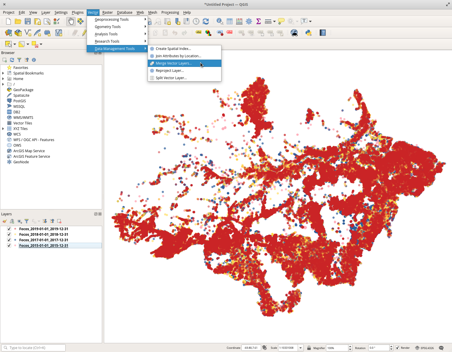
The first task was to visualize those 350,000 fire points for 2016–2019 as a heatmap. After downloading the fires for each year as shapefiles from the BDQueimadas platform (which is maintained by INPE — the Brazilian National Institute for Space Research), I opened them in QGIS. Since each row already had a timestamp string variable called datahora, I was able to use the QGIS field calculator to pull out the year substring for a new year variable. QGIS has a feature to merge shapefiles called ‘Merge Vector Layers’, which I used to make one shapefile with data from all four years.

Next, using ogr2ogr in the command line, I converted that consolidated shapefile to a GeoJSON file. The command looks something like this:

ogr2ogr -f GeoJSON allfires.geojson allfires.shp

A GeoJSON file with this many points is much too big to quickly load in the browser, so I needed to convert that file once again. This time I converted it to a vector tiles .mbtiles file, a format supported by the Mapbox Studio platform. Mapbox itself created a tool for converting GeoJSON files to vector tiles: tippecanoe. The tippecanoe command I used looked like this:

tippecanoe -zg -o allfires.mbtiles — drop-densest-as-needed allfires.geojson

With that, I was able to upload the data source (allfires.mbtiles) to my Mapbox Studio account, which automatically generated a data source URL for me. Mapbox.GL has built-in functionality to display point data as a heatmap. I added a new layer to my Mapbox.GL map (using their JavaScript API) with the following heatmap paint properties:

I also created a slider to filter the fire data by year, using the ‘year’ variable that I added while organizing the data in QGIS.

Deforestation Data Layer

I followed a very similar set of steps to create the deforestation layer on the map. Deforestation data from the Amazon region is also available from INPE, and is freely downloadable from the Terra Brasilis platform. The dataset used to describe deforestation per year is called PRODES, and it uses the time period of August of the previous year to July of the current year to summarize the deforestation season. For example, the total for 2019 actually includes all deforestation that happened between August 2018 and July 2019.

The only caveat to this was the data for deforestation in 2020. Because PRODES data is only published after the year is done, I used a different INPE data source, DETER, to map deforestation in 2020. DETER deforested area polygons are published each month, although they are not as precise as PRODES data and often underestimate the total deforestation between the months of August and July by 30–40%.

Municipalities Data Layer

To describe the relationship between deforestation and fires at the municipal level, I knew I wanted to create a bivariate choropleth map. First, I used QGIS to clip a shapefile of municipalities of Brazil (published by IBGE, the Brazilian Institute of Geography and Statistics) to the legally defined Amazon region. Deforestation data per municipality was already available as a .csv file export from INPE on the Terra Brasilis platform, under ‘Municipalities per State Tool’.

I still needed to count fires per municipality, however. I used the QGIS ‘Count Point in Polygon’ tool to count how many 2019 forest fires occurred within each of the Amazon municipalities. Now I had two new variables per municipality polygon — one for 2019 deforestation and one for 2019 fires. This tutorial was a fundamental guide to how to create the necessary fields and colors in QGIS.

I converted the resulting file to GeoJSON and then vector tiles once again. To bring it all together, I hard-coded the bivariate choropleth breakpoints and color palette values for the Mapbox.GL layer.

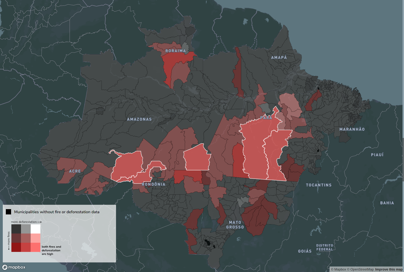
The legend for this layer needed a little more detail than a simple SVG shape, so I used Vega to create a mini grid of colors. There are two color gradients — one from dark gray to white to represent deforestation values, and one from dark gray to red to represent fires. The brightest, reddest color values show the municipalities with high values for both fire counts and deforested areas.

Rural Properties Data Layer

The data for the rural properties data layer came from SICAR, the Brazilian Forest Service, from a dataset called CAR — the Rural Environmental Registry. This data contains official records of all registered rural properties throughout Brazil, organized by municipality. After finding that the same four municipalities that topped the list for deforested km2 also topped the list for fire counts, I downloaded the shapefiles of properties from CAR for each of them.

Next, I used the QGIS field calculator once again to assign a value to each polygon based on whether the property was larger than 440 acres. Different municipalities categorize the size of properties differently. Most classify properties as ‘large’ if they are 4 fiscal units or greater, but the size of a fiscal unit varies in different municipalities and states. The largest possible size for a single fiscal unit is 110 acres, so we chose 440 acres as the cut-off point for small to medium properties.

Putting It All Together

Most of the layers were available as shapefiles, so they needed to be converted to GeoJSON to be compatible with tippecanoe so that I could turn them into vector tiles. Once they were all in the .mbtiles format, I uploaded the files to Mapbox Studio, and then imported them into Mapbox.GL as data sources. To see the code itself, check out the Observable Notebook.

Useful articles:

Data Sources: